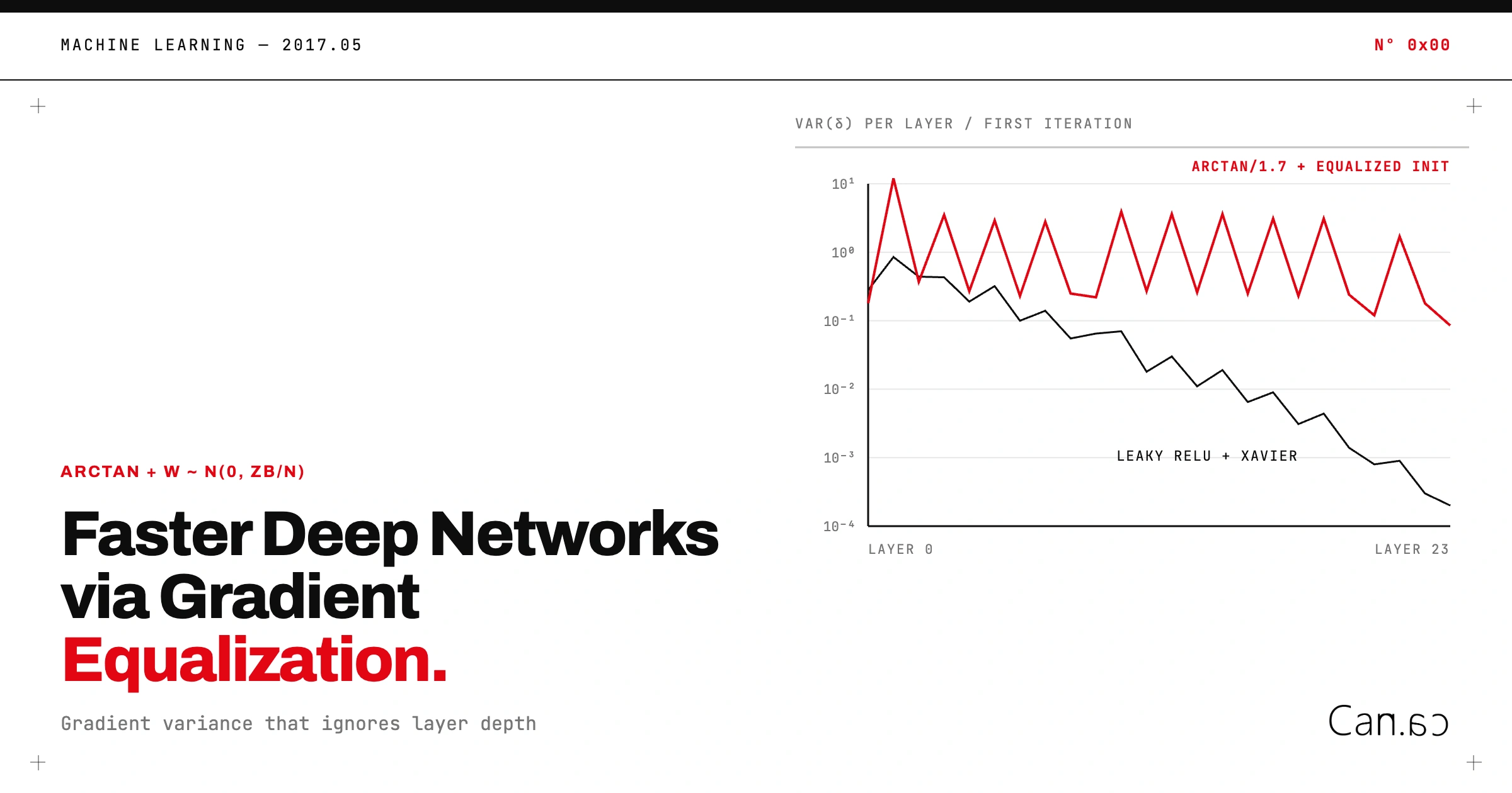
Faster Results with Deep Neural Networks via Gradient Equalization
When I was 17, I wrote this paper and, armed with the unshakeable confidence only a teenager can have, tried to get it into a journal. Here it is.
The original version is available as a PDF.
0x0: Abstract
The field of machine learning has been dominated by deeper and deeper neural networks ever since rectified linear activation functions became commonplace instead of their non-linear, bounded, counterparts such as sigmoid or hyperbolic tangent. Regardless of this major change, deep neural networks still take much longer to train compared to their shallow alternatives. After examining the rationale behind using deeper neural networks, our objective is to investigate the cause of this problem and come up with a solution by manipulating the gradients. We propose an initialization technique that when used in combination with a smoother activation function such as arctan, keeps the variation and expected value of the gradients at a similar level for all layers regardless of the depth of the network. This allows us to train deeper networks in much less time and use bounded activators without worrying about the problem of vanishing or exploding gradients.
0x1: Introduction
Artificial neural networks (ANNs) are complex modelling techniques that can be used to find the relation between the output of a complex multi-variable function and its arguments, effectively approximating it.
Nowadays, ANNs are being used successfully for a variety of tasks ranging all the way from predicting liver cancer[1] and approximating physics of fluids[2] to autonomous vehicles and colourizing black and white videos[3]. Neural networks require many layers to be stacked for such complex classification and prediction problems as they need to develop complex feature detectors for the data used for these tasks.
Apart from the fact that computation power and memory required increases as layers get stacked up, there is also architectural issues that make training deep neural networks (DNNs) hard, such as vanishing/exploding gradients and numerical instabilities.
As a way to address the vanishing gradient problem, researchers working in the field of machine learning have been using rectified linear units (ReLUs)[4] such as \(max\{x,0\}\) with Xavier initialization[5].
Although gradients vanish much slower when ReLUs are used compared to exponentially increasing activators (e.g., sigmoid, tanh), it is not the only way to approach the issue and it almost definitely is not a perfect solution. ReLUs not only have many cons of their own such as dying units[6] and exploding gradients but also do not completely fix the vanishing gradient problem which will be demonstrated later in Section 1.2.
The primary concern of this paper is to accelerate deep neural networks’ training phase further and address the numerical problems with gradients at the same time. We propose a weight initialization technique that lets us stack up layers and have “gradient-equalized” layers when combined with soft activation functions. This enables us to use much deeper networks without the need of a recurrent architecture.
1.1 Rationale Behind Using Deeper Networks
Nowadays, almost all state of the art results in complex image classification, object detection and semantic segmentation problems are achieved using very deep neural networks. One example would be GoogLeNet[7] with 22 convolutional layers. This is simply because of the fact that shallow neural networks sacrifice accuracy and complexity for ease of training, but they are not very suitable for everyday use due to this. With fields that use neural networks for complex recognition tasks such as autonomous driving or cancer prediction, sacrificing feature complexity is simply intolerable.
We can easily prove this claim of “shallow” networks sacrificing the ability to form more complex models by testing it using a regression task.
We trained neural networks with 2, 4 and 12 layers on NVIDIA’s stock value for last 200 days, normalized using Equations \(\ref{eq_normx}\) and \(\ref{eq_normy}\).
$$ \begin{align} \hat{x} := \frac{x}{\max X} \label{eq_normx} \end{align} $$$$ \begin{align} \hat{y} := \frac{y - E[Y]}{\sqrt{Var[Y]}} \label{eq_normy} \end{align} $$After the training has been done as we needed to measure the complexity of networks’ output in a quantitative way and both our input and output were 1 dimensional, we measured the complexity of the features by graphing the input and output of the network, computing the numerical derivative for every point on the predicted line and then calculating the array’s variance like in Equation \(\ref{eq_complexity}\).
$$ \begin{align} \theta = Var\{ y'(0), y'(0.1), \ldots \} \label{eq_complexity} \end{align} $$| Number of Layers | \(\theta\) | \(\frac{\theta}{\min\theta}\) |
|---|---|---|
| 2 | 0.000063 | x1.000 |
| 4 | 0.000977 | x15.460 |
| 12 | 0.002224 | x35.206 |
Referring to Table 1, the 12-layer network developed features that are \(\approx\)35 times more complex compared to the 2-layer network in 125'000 iterations.
1.2 Examination of the Problem
It is widely known that deep neural networks have problems with unstable gradients. As a solution, ReLUs are being used by many researchers, however, ReLUs do not completely fix this issue by any means as we will demonstrate and it ends up creating new issues such as dying units and exploding gradients.
In order to test whether ReLUs completely eliminate the vanishing gradients problem, we used a convolutional neural network with 8 convolutions and 3 fully-connected layers. We initialized the weights using Xavier initialization, and once the first iteration is finished we logged every gradient to a file and analysed its distribution.
In Figure 2 the point \(x=22\) on both graphs shows us the last weight layer’s distribution. We can see that even though ReLU was used as the activator, variance of the gradients in the last weight layer reached values lower than \(0.0002\) and mean kept decreasing steadily indicating the problem was not solved.
0x2: Hypothetical Solution
In order to solve the problem of gradient instability we first need to define the problem mathematically. The problem with unstable gradients can be defined as gradients either exploding or vanishing after passing one weight and one activation layer. We will assume it is a fully-connected layer for the sake of ease. The value after passing these two layers can be defined as in Equation Set \(\ref{eq_neuron_act}\) where f is the activation function, x is the input, y is the activated final output and w is the weight of the particular connection.
$$ \begin{align} \begin{split} a_{i} &= \sum_{n}^{} x_{n} w_{n \rightarrow i} \\ y_{i} &= f(a_{i}) \end{split} \label{eq_neuron_act} \end{align} $$Let \(\delta_n = \frac{\partial E}{\partial y_{n}}\) where E is the error function, how \(\delta_n\) effects the gradient \(\frac{\partial E}{\partial x_{z}}\) can be seen in Equation \(\ref{eq_neuron_bprop}\).
$$ \begin{align} \begin{split} \frac{\partial E}{\partial x_{z}} &= \sum_{n}^{} \frac{\partial E}{\partial y_n}\frac{\partial y_n}{\partial x_z} \\ &= \sum_{n}^{} \delta_n f'(a_{n}) \sum_{k}^{} \frac{\partial}{\partial x_z} \bigg[ x_{k} w_{k\rightarrow n} \bigg] \\ &= \sum_{n}^{} \delta_n f'(a_{n}) w_{z \rightarrow n} \end{split} \label{eq_neuron_bprop} \end{align} $$We want Equation \(\ref{eq_var_fix}\) to hold true to achieve our goal of equalizing the gradients. In order to evaluate Equation \(\ref{eq_var_fix}\) we are going to make the original assumption of gradients having zero mean from Xavier initialization, \(E[f'(a)]=0\), and then use Bienaymé formula.
$$ \begin{align} \begin{split} Var\bigg[ \frac{\partial E}{\partial y_{n}} \bigg] &= Var\bigg[ \frac{\partial E}{\partial x_{n}} \bigg] \\ Var[\delta_n] &= Var\bigg[ \sum_{n}^{} \delta_n f'(a_{n}) w_{z \rightarrow n} \bigg] \\ Var[\delta_n] &= \sum_{n}^{} Var\bigg[ \delta_n f'(a_{n}) w_{z \rightarrow n} \bigg] \\ 1 &= n Var[ f'(a) ] Var[ w_{z} ] \end{split} \label{eq_var_fix} \end{align} $$We still cannot solve this for \(Var[ w_{z} ]\) as it still contains the unknown variable \(a\). So we are going to assume \(Var[f'(a)] = \max\limits_{x \in {\rm I\!R}^n} Var[f'(x)]\) in order avoid having exploding gradients.
$$ \begin{align} Var[ w_{z} ] = \frac{1}{n} \frac{1}{\max\limits_{x \in {\rm I\!R}^n} Var[ f'(x) ]} \label{eq_var_fix2} \end{align} $$We will simplify things a little bit more and solve Equation \(\ref{eq_var_fix2}\) in terms of \(\frac{Z}{n}\). Distribution wise we can simplify the tensor transformed by \(f'\) of any dimension that has the maximum variance to \(\{ \max f'(x), \min f'(x) \}\). As the final solution we have the Equations \(\ref{eq_var_fix_e1}\) and \(\ref{eq_var_fix_e2}\) where \(\beta\) is the hyper parameter defining the controlled drop coefficient which we use to ensure the creation of higher level feature detectors in deeper layers.
$$ \begin{align} Z = \frac{1}{Var\{ \max f'(x), \min f'(x) \}} \label{eq_var_fix_e1} \end{align} $$$$ \begin{align} W \sim \mathcal{N} \bigg( 0, \frac{Z}{n} \beta \bigg) \label{eq_var_fix_e2} \end{align} $$2.1 Activaton Function
One problem that remains is the activator function. As universal as the solution in Equation \(\ref{eq_var_fix_e2}\) sounds, it cannot used with non zero-meaned or strict activators like sigmoid or tanh, nor with functions that do not follow the rules of Universal Approximation Theorem[8].
We will declare weights where \(f'(w) < 0.001\) “slow”, and visualize the problem. As it can be seen in Figure 3, when we use tanh as the activator, \(\approx 4\%\) of the network is learning “slowly” when there is only one layer. This effect increases exponentially as the number of layers increase.
Instead of an exponentially increasing function like sigmoid or tanh, we are going to use arctan which increases quadratically and squash it using a hyper-parameter, \(\gamma\) as seen in Equation \(\ref{eq_arctan}\).
$$ \begin{align} f(x) = \frac{1}{\gamma} \arctan(x) \label{eq_arctan} \end{align} $$As it can be seen from the 2nd and 3rd graphs of Figure 3, due to its quadratically increasing nature, the proposed activator did not experience the issue tanh activator did even though the variation was much higher with arctan.
0x3: Experimental Setup and Datasets
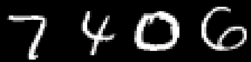
We are going to be using MNIST (Figure 5), STL-10 (Figure 6) and a custom dataset (Figure 7) when benchmarking our technique and compare it with other techniques. STL-10 is a particularly interesting challenge as it only contains 500 images per class.


As all of these tasks are classification tasks, cross entropy will be used and every network will be regularized using L2 regularization with regularization coefficient \(\lambda = 10^{-4}\). All benchmarks will be done using a custom CUDA library and GTX 1080.
0x4: Results
Before starting other tests we decided to search for the most optimal value for \(\gamma\) from the set \(\big[1.1, 1.2, \dots, 1.9\big]\). For each value of \(\gamma\), we trained 25 networks for 20000 iterations on MNIST dataset and averaged the cross-entropy loss.
Although we originally thought \(\gamma=\pi/2\) would be the best fit, constraining the output to [-1, +1] precisely, this was not the case as seen from Figure 9. Going from \(\gamma=1.1\) to \(\gamma=1.9\), error almost halved due to higher values of \(\gamma\) allowing higher variance. As a result, we will be using \(\gamma=1.7\) for our tests.
4.1 Analysis of the Gradients
For the first test, we checked whether the technique we proposed circumvents the problem of unstable gradients as expected or not. For comparison, we are going to use the network from Figure 2.
As it can be seen from Figure 8, neither variance nor the mean of gradients shows any correlation with the depth of the layer.
The see-saw behaviour of both graphs are due to the fact that the Z value we used for the variance of the weight tensor bumps up the variance in a way that when the activation function squishes the input (thus lowering the variance), the variance returns to the exact same previous level which means our technique works as we expected; preventing the gradients from vanishing.
We tested whether this assumption was correct or not by training a network on XOR dataset. In our tests, we were not able to train a 30-layer feed forward network for XOR dataset with traditional methods within 100k iterations whereas our technique reached \(\approx 5\%\) error by 2000 iterations.
4.2 Effect of β hyper-parameter
In order to see the effect of \(\beta\) on training accuracy, we trained 3 networks with \(\beta\) values set to 0.5, 0.7 and 1.0 on STL-10 dataset. As it can be seen from Figure 10, although the difference between 0.5 and 0.7 is hard to interpret, it is rather apparent that values other than 1.0 had better validation and training accuracy. This leads us to believe that \(\beta\) value should be included in hyper-parameter search when setting up the network as it depends on the network’s architecture and complexity of the data used.
4.3 Feature Complexity and Visualization of Learned Features
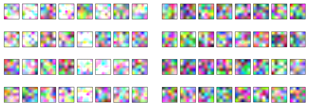
Gradient-equalization affects the development of features in a rather interesting way. When the gradient drops as layers go like in a traditional network, the filters get more complex as the layer gets deeper. On the other hand, when our method is used, complexity is distributed across layers; achieving a highly-complex network rather than highly-complex deep layers.
Figure 11 visualizes first layer of a network trained on STL-10 dataset before and after training phase. As it can be seen, although some features were certainly learned, it can not be easily interpreted unlike traditional networks except for a few line patterns.
This approach sacrifices the possibility of transfer learning and ease of visualizing for speed and overall complexity. It also makes it easier for these networks to over-fit training dataset but this is not as big of a problem as we thought originally since our network were able to achieve similar results to 2012 (supervised) state of the art[11] within 8 epochs on STL-10 dataset which contains only 500 images per class.
4.4 MNIST Dataset
For the first experiment we conducted, we used MNIST as it was the easiest dataset of all 3. As it can be seen from Figure 12, it took 25 epochs for the network using traditional techniques to reach the accuracy network using our technique reached in 3 epochs. Our network ended up reaching 98.44% validation accuracy by the end of 23 epochs.
4.5 STL-10 Dataset
This dataset is especially interesting because it has less data when compared to CIFAR-10[12] and yet 9 times the input volume. We compared the performance of our network to the results of StochasticNet[13] published in 2015. It can be seen from Figure 13 that our network reached \(\approx\)40% accuracy within a single epoch whereas other networks took 5 epochs and our network reached \(\approx\)56% accuracy within 9 epochs whereas it took StochasticNet 18 epochs, and ConvNet could not reach it within 20 epochs. Our network ended up reaching 61.68% validation accuracy by the end of 20 epochs.
4.6 Our Dataset
We used a custom dataset in order to compare the performance for fast learning when the input data is large (96x96x3) but the pattern is easy to recognize. Our method performed significantly better reaching \(\approx 4\%\) validation error within 3 epochs with only 2000 actual examples in training set and 1000 examples in validation set whereas the traditional methods could only reach \(\approx 49\%\) error rate within this very short time as it can be seen from Figure 14. Our network ended up reaching 99.76% validation accuracy by the end of 20 epochs.
4.7 Performance
Although ReLUs are known for being especially fast as they do not require floating-point computations like arctan, sigmoid or tanh, we noticed in our tests that our model actually ran 5% faster compared to ReLUs. We assume this is because of the fact that our activator does not require any branching unlike ReLUs as GPUs are rather bad when it comes to branches due to the fact that they require both paths to be executed by all the threads when there is branch divergence within a warp.
4.8 Conclusion
Results from the training phases of these datasets certainly provided us concrete proof that our technique lets deep neural networks reach high training and verification accuracies much faster compared to the traditional techniques. For the networks where our technique was used, the speed of learning was affected by the complexity of dataset rather than the depth of the network as all layers of the network trained at similar speeds.
Our technique also had the benefit of human-like learning where network learned the basics of the dataset (this basic knowledge covered \(\approx\)85% of the dataset for MNIST and our dataset and \(\approx\)40% of the dataset for STL-10) very fast (within a single epoch) and got better at it eventually, letting us have the best of both worlds — accuracy and speed.
0x5: Future Work
One question that still remains is whether the controlled gradient drop technique we used were satisfactory or not. After calculating the \(\beta\) hyper-parameter which would drop the gradient to \(1/10\)th of the original in the first layer, we saw that although the ratio between first and final layer were certainly \(1/10\), the hidden layers did not necessarily follow the exponential drop we wanted perfectly, as it can be seen from Figure 15.
References
- Q.-H. Ye, L.-X. Qin, M. Forgues, et al., “Predicting hepatitis b virus–positive metastatic hepatocellular carcinomas using gene expression profiling and supervised machine learning,” Nature medicine, vol. 9, no. 4, pp. 416–423, 2003.
- J. Tompson, K. Schlachter, P. Sprechmann, and K. Perlin, “Accelerating eulerian fluid simulation with convolutional networks,” arXiv preprint arXiv:1607.03597, 2016.
- S. Iizuka, E. Simo-Serra, and H. Ishikawa, “Let there be color!: Joint end-to-end learning of global and local image priors for automatic image colorization with simultaneous classification,” ACM Transactions on Graphics (TOG), vol. 35, no. 4, p. 110, 2016.
- V. Nair and G. E. Hinton, “Rectified linear units improve restricted boltzmann machines,” in Proceedings of the 27th international conference on machine learning (ICML-10), 2010, pp. 807–814.
- X. Glorot and Y. Bengio, “Understanding the difficulty of training deep feedforward neural networks.,” in Aistats, vol. 9, 2010, pp. 249–256.
- K. He, X. Zhang, S. Ren, and J. Sun, “Delving deep into rectifiers: Surpassing human-level performance on imagenet classification,” in The IEEE International Conference on Computer Vision (ICCV), Dec. 2015.
- C. Szegedy, W. Liu, Y. Jia, et al., “Going deeper with convolutions,” in Proceedings of the IEEE Conference on Computer Vision and Pattern Recognition, 2015, pp. 1–9.
- A. R. Barron, “Universal approximation bounds for superpositions of a sigmoidal function,” IEEE Transactions on Information theory, vol. 39, no. 3, pp. 930–945, 1993.
- C. J. Burges, Y. LeCun, and C. Cortes, “Mnist database,” [Online]. Available: http://yann.lecun.com/exdb/mnist/.
- A. Coates, H. Lee, and A. Y. Ng, “An analysis of single-layer networks in unsupervised feature learning,” Ann Arbor, vol. 1001, no. 48109, p. 2, 2010.
- Y. Jia, C. Huang, and T. Darrell, “Beyond spatial pyramids: Receptive field learning for pooled image features,” in Computer Vision and Pattern Recognition (CVPR), 2012 IEEE Conference on, IEEE, 2012, pp. 3370–3377.
- A. Krizhevsky and G. Hinton, “Learning multiple layers of features from tiny images,” 2009.
- M. J. Shafiee, P. Siva, and A. Wong, “Stochasticnet: Forming deep neural networks via stochastic connectivity,” arXiv preprint arXiv:1508.05463, 2015.
Appendices
A.1 Network Used for STL-10 and Our Dataset
 1Convolution [96, 96, 3] → [94, 94, 32] (3x3)
 2Activator Arctan * 1/1.7
 3Convolution [94, 94, 32] → [92, 92, 32] (3x3)
 4Activator Arctan * 1/1.7
 5Pool [92, 92, 32] → [46, 46, 32] (2x2)
 6Convolution [46, 46, 32] → [44, 44, 64] (3x3)
 7Activator Arctan * 1/1.7
 8Convolution [44, 44, 64] → [42, 42, 64] (3x3)
 9Activator Arctan * 1/1.7
10Pool [42, 42, 64] → [21, 21, 64] (2x2)
11Convolution [21, 21, 64] → [19, 19, 128] (3x3)
12Activator Arctan * 1/1.7
13Convolution [19, 19, 128] → [17, 17, 128] (3x3)
14Activator Arctan * 1/1.7
15Pool [17, 17, 128] → [8, 8, 128] (3x3)
16Convolution [8, 8, 128] → [6, 6, 256] (3x3)
17Activator Arctan * 1/1.7
18Convolution [6, 6, 256] → [4, 4, 256] (3x3)
19Activator Arctan * 1/1.7
20Pool [4, 4, 256] → [2, 2, 256] (2x2)
21Fully Connected [2, 2, 256] → [1024, 1, 1]
22Activator Arctan * 1/1.7
23Dropout p=0.5
24Fully Connected [1024, 1, 1] → [1024, 1, 1]
25Activator Arctan * 1/1.7
26Fully Connected [1024, 1, 1] → [1024, 1, 1]
27Activator Arctan * 1/1.7
28Dropout p=0.5
29Fully Connected [1024, 1, 1] → [10/6, 1, 1]
30Softmax
Beta, momentum, learning speed and batch-size were grid-searched. Learning speed were multiplied with 0.2 once the network’s error started to plateau.
A.2 Network Used for MNIST
 1Convolution [28, 28, 3] → [26, 26, 64] (3x3)
 2Activator Arctan * 1/1.7
 3Convolution [26, 26, 64] → [24, 24, 64] (3x3)
 4Activator Arctan * 1/1.7
 5Convolution [24, 24, 64] → [22, 22, 64] (3x3)
 6Activator Arctan * 1/1.7
 7Convolution [22, 22, 64] → [20, 20, 64] (3x3)
 8Activator Arctan * 1/1.7
 9Pool [20, 20, 64] → [10, 10, 64] (2x2)
10Convolution [10, 10, 64] → [8, 8, 128] (3x3)
11Activator Arctan * 1/1.7
12Convolution [8, 8, 128] → [6, 6, 128] (3x3)
13Activator Arctan * 1/1.7
14Convolution [6, 6, 128] → [4, 4, 128] (3x3)
15Activator Arctan * 1/1.7
16Convolution [4, 4, 128] → [2, 2, 128] (3x3)
17Activator Arctan * 1/1.7
18Fully Connected [2, 2, 128] → [512, 1, 1]
19Activator Arctan * 1/1.7
20Dropout p=0.5
21Fully Connected [512, 1, 1] → [512, 1, 1]
22Activator Arctan * 1/1.7
23Dropout p=0.5
24Fully Connected [512, 1, 1] → [10, 1, 1]
25Softmax
Beta, momentum, learning speed and batch-size were grid-searched. Learning speed were multiplied with 0.2 once the network’s error started to plateau.